Efficiently projecting large number of nodes with GDS

[mranand4]

So, my graph is modeled for retail transactions and it's fairly large - 250M nodes. Nodes in my graph are bidirectionally connected and are as follows:

1. Customer (Has an outgoing edge to Transaction, Has an incoming edge from Transaction) (Red color)
2. Card (Has an outgoing edge to Transaction, Has an incoming edge from Transaction) (Pink)
3. Transaction (Has an outgoing edge to Card, Customer, Has incoming edge from Card, Customer) (Blue with transaction amount) (150M nodes)
   
   

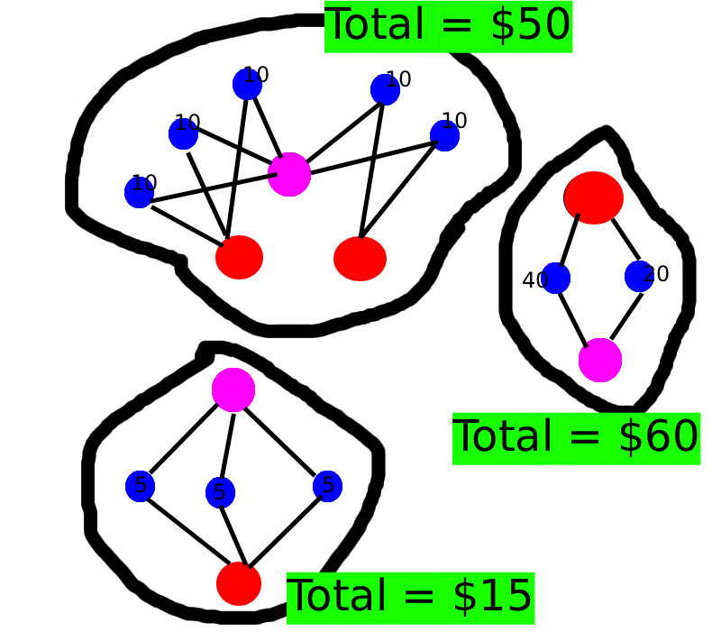
I am interested in knowing the components for which the total transaction amount is largest -- basically top n components by transaction amount. E.g. in the above figure component with $60 > $50 > $15. For this I'm using Graph Data Science library in conjunction with APOC.

However, since the data size is quite large in my case, the "graph projection" itself is taking too much time. It's taking around 7-8 hours to project all 150M nodes. Overall heap memory for the projection is ~10GB. Running gds.wcc.stream which then takes 10-15 mins to find the largest component. I want to know how I can further optimize my projection query to speed up my projections. Here's the query which I'm using to project my graph:

// Note I'm running this query over and over again from my java app until the graph is fully projected fully.
// In one query execution, some 500k nodes are projected from a "seed" of 50k nodes.
// I didn't used LIMIT before but it was way too slow, also with LIMIT I can mark the already visited nodes and don't visit them again for projection. 

// Since transaction amount is in Transaction node, I'm only projection this node
MATCH (n:Transaction)
WHERE NOT n:AlreadySeen // Don't consider nodes which have been projected before
WITH n
LIMIT 50000
SET n:AlreadySeen // Mark the node as seen
WITH n

// I want to find all the transactions in a components -- basically all the Transaction nodes which I can reach starting from a given seed Transaction node
// I tried cypher before
// (n)-[*]->(m:Transaction)
// but apoc is somewhat faster
CALL apoc.path.subgraphNodes(n, {
  minLevel: 1,
  maxLevel: 299, // I've some pretty big components/clusters,
  relationshipFilter: ">" // forward direction works given the nature of o
}) YIELD node
// Again, checking if it was not already seen before and filtering only transaction nodes
// Also, I am only target online transactions
// I have indexed transaction_mode field
WHERE (NOT node:AlreadySeen AND node:Transaction AND node.transaction_mode="ONLINE"

// marking the reachable transaction nodes as AlreadySeen so we don't consider them in further iterations
SET node:AlreadySeen

WITH COLLECT([n, node]) AS distinct_pair_list // apoc gives distinct nodes only?
UNWIND distinct_pair_list AS pair

// I'm setting the graph name from the java app ... this is just a dummy name
WITH gds.graph.project("project_graph_1", pair[0], pair[1]) AS g
RETURN {
 projection_name: g.graphName,
 node_count: g.nodeCount
}

Again, I've to run this query like 400 times to project 400 minigraphs. Then I find top 10 components by transaction amount in each of those 400 projections and put them into a list. From the list, I then pick actual top 10 transactions! Welp!

I want to know what I can do further improve my projection times? Should I add a filter for only "ONLINE" transactions in the first MATCH as I only want those? I am using neo4j community at the moment and can't scale beyond 4 threads.

Thanks in advance !!!

EDIT

This query projects the entire graph with this is very fast but takes ~20GB heap

CALL gds.graph.project("project_graph_1", "*", "*") YIELD graphName, nodeCount, relationshipCount

Is there any way to project just Transaction nodes? I don't really understand why projecting all the nodes is faster than projecting just Transaction nodes. Likely because of all the traversals I'm doing in my initial query?

[finbar.good]

I have a couple of suggestions that might work for you:

Use your schema to find a starting point for each cluster

You have chosen transactions as your starting point for finding pairs of transaction in the same cluster. I am guessing that either Card or Customer nodes are much less numerous. Picking Customer as a starting point, it is possible to find all other reachable Customer nodes i.e. Customer nodes in the same cluster. With a bit of ingenuity using ordering and reduce, we can pick a root Customer node for each cluster:

MATCH (c1:Customer)-->{0,299}(c2:Customer)
  WHERE c1 <= c2

// DISTINCT enables an efficient plan
WITH 
  c1 AS head,                                             
  collect(DISTINCT c2) AS members  
  ORDER BY head  
WITH collect({head: head, members: members}) AS sets

// At this point we have multiple sets of Customers per cluster
// This reduce picks the largest set for each cluster. It works because above we
// used c1 <= c2 and ORDER BY to ensure the largest set per cluster is first
WITH reduce(
  acc = { sets: [], seen: []},
  set IN sets | 
    CASE 
      WHEN set.head IN acc.seen THEN acc 
      ELSE { sets: acc.sets + [set.members], seen: acc.seen + set.members }
    END ).sets AS sets
UNWIND sets AS set

// We only need one Customer node per cluster as a starting point
WITH head(set) AS rootCustomer

rootCustomer can be used as a single starting point for finding all Transaction nodes in the same cluster.

Use plain Cypher to find the clusters and calculate the total

I am not sure if you are using WCC for something else but at this point you are just a short step from doing the calculation:

MATCH (rootCustomer)-->{1,299}(tnx:Transaction {transaction_mode: "ONLINE"})
WITH rootCustomer, collect(DISTINCT tnx) AS cluster
RETURN reduce(acc = 0.0, node IN cluster | acc + node.amount) AS totalAmount

You can then ORDER and LIMIT to get the top N clusters by amount, and you can pick your sample transactions from cluster as needed.

If you want to project these to GDS instead, then you can adapt it like this:

MATCH (rootCustomer)-->{1,299}(tnx:Transaction {transaction_mode: "ONLINE"})
WITH head(cluster) AS root, tail(cluster) AS tail
UNWIND tail AS node
WITH gds.graph.project("project_graph_1", root, node) AS g
RETURN {
 projection_name: g.graphName,
 node_count: g.nodeCount
}

[mranand4]

Thanks, you are correct in assuming that both Card and Customer nodes are much less numerous. The approach which you suggested is pretty smart and I modified my query to start with Customer nodes.

But, while it's faster than my original approach, it still doesn't compares with projecting the entire graph with gds via gds.graph.project("project_graph_1", "*", "*"). Projecting entire graphof 250M nodes takes only a minute and than 5 more minutes to give me the top online components with this

CALL gdc.wcc.stream("project_graph_1") YIELD nodeId, componentId
WITH gds.util.asNode(nodeId) AS node, componentId
WITH COLLECT (DISTINCT node) AS nodes, componentId
WITH nodes, componentId, REDUCE
(
  total_online_amt = 0,
  n IN nodes |
    total_online_amt + 
      CASE
        WHEN n:Transaction AND n.transaction_mode="ONLINE"
           n.amount
       ELSE
          0
       END
) AS total_online_amount

ORDER BY total_online_amount DESC 
LIMIT 10

RETURN {
  component_id: componendId
  total_online_transaction: total_online_transaction
}

I somehow missed to try this approach first and started with a more complex solution .

However, I am now interested in knowing why projecting entire graph is faster than projecting only nodes of a certain type/label. I'm guessing it's because of some under the hood optimizations done by n4j.

[mranand4]

I'm interested in knowing a couple of more things.

1. Memory estimate of projecting the entire graph with gds.graph.project.estimate( "*", "*") is 17GB ... 19GB, however this increases when I try to project only select nodes - gds.graph.project.estimate({Card: ["amount"], Customer: ["customer_id"]} to 24 ... 25GB. I presumed that memory estimation will be lower in the query projection given that it has only two nodes and only absolute essential properties. But contrary to my assumption -- the memory estimation is much more ... do you know why n4j behaves in this way?
2. How can I project all the nodes but only keep certain properties in them? I'm trying to reduce my memory consumption and thought projecting lesser properties might help.